I am not very found of language theory. It is a difficult topic, and I am not very good at it, to be honest. Do not ask me about derivation, reductions and so on, it does not even make sense to me!
However, there is an aspect of languages that I find fascinating, and that is the parsing aspect. I like building lexers and parsers, especially parsers, and there is one technology that I particularly find interesting: parser combinators.
The principle behind parser combinators is to provide simple parsers with simple tasks (“atomic” parsers) and combinators, that is, ways of combining the simple parsers to build more complex parsers.
In this article, I will try to cover what is a parser, what are combinators, and how to implement them in Haskell. The choice of Haskell will become self-evident when we get to it, but as hinted by the title, the language’s inherent laziness is a key ingredient for defining recursive parsers.
Parsers and parsers combinator
A parser can be defined as a box that takes as input a stream of characters and outputs either some result and the remainder of the stream, or a failure.
Basically, this box is able to “recognize” a particular character or set of characters in the stream, extract it and calculate a result from it; or, if it cannot recognize it, yields a failure.
Of course, I am talking about “streams” and “characters”, but one can imagine parsers for any kind of sequential structure and for any kind of data (numbers, tokens, and even complex structures, why not!).
The concept of success and failure for parsers is essential for parser combinators. One may have recognized that the result of a parser is basically a monad, but we are getting ahead of ourselves.
For now, let us imagine a stream of symbols, for example letters (A, B, C, …) and the parser that recognizes the symbol A and returns the number 10 when it does.
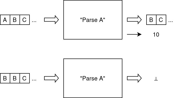
Parse A &endash; Possible outcomes
As you can see on the figure, recognizing symbol A yields the intended result (10) and also the remainder of the stream, excluding what was recognized. Failing to recognize a symbol, the parser yields ⊥ (bottom or up-tack), which symbolizes failure.
Combinators
You may have noted that a parser inputs and (sometimes) outputs a stream, in addition to its result. The natural thing a computer scientist (or a plumber) might want to do next is to plug the output of the parser into the input of another one, like so;
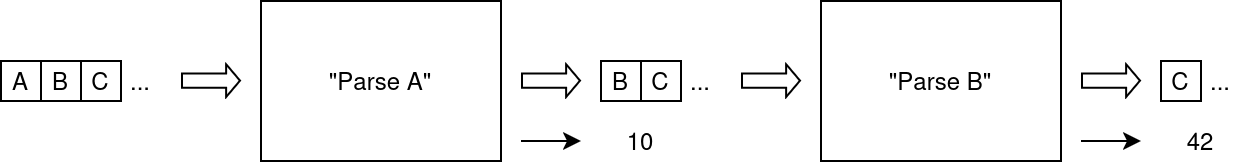
Chaining 'Parse A' and 'Parse B'
Intuitively, by “chaining” two parsers (here, the one that parses A and then the one that parses B), we obtain what looks (or behaves) like a box that takes a stream of symbols as input and outputs a result and the remainder of a stream; in other words, we got a new parser!
Now how does that parser behave? Well when the first parser fails, the second does not get its input stream, so it fails as well. If the first succeeds, then the second gets its input stream and parses it; the result of that stream is what ends up being output.
In the example above, the first parser succeeds in parsing A from ABC… and outputs 10 and BC…; then the second parser succeeds in parsing B and outputs its own result (42) and the remainder C… (what happens to the first result is a matter of “taste”: it may be composed with the second result, or discarded altogether, we will see what this entails later).
Put an other way, the resulting parser has parsed AB and output the result of the second parser. That is: it parsed the sequence of what each parser parses, in order. For this reason, this construction may be called sequencing.
Now we took two parsers and built a new parser using a general construction. This construction is said to be higher order, and we call it a combinator. And, because it takes parsers as input and yields a parser as output, we may call it a parser combinator!
Let’s explore another way we can combine parsers.
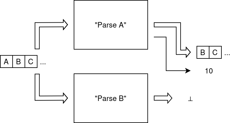
'Parse A' and 'Parse B' in 'parallel'
In this combinator called alternative, the stream is presented at the input of both parsers. If both parser fails, then the resulting parser fails. Otherwise, if one of the parser succeeds, then its result is presented to the output. If both parser succeed, we take one of the result arbitrarily (usually we chose the result of the first one).
Basically, in the example above, what we end up parsing is either A or B, thus this is why we call it alternative.
One last combinator I want to talk about is the repetition combinator:
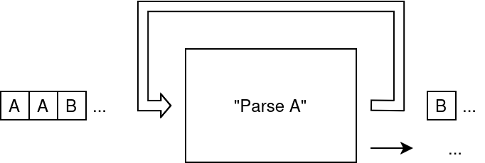
'Parse A' repeated
This one is maybe a bit more tricky to grasp. Basically, a repeated parser always succeed. It “runs” the parser as much as possible until it fails, an returns the aggregated result (again, a matter of taste).
In the example above, let us say we have a stream of five A. Then the repeated parser will parse A five times, and succeed with the resulting stream, which is composed of the remainder after the five A. Note that the repeated parser succeeds as well if the stream contains no A, an leaves the stream untouched. Basically, the parser got “triggered” 0 times, which is allowed.
Atomic parsers and notations
As mentioned earlier, combinators work by combining parsers. The idea then is to build a complex parser by applying combinators, starting with small, simple parsers with a simple task, that I like to call atomic parsers.
We have already seen one atomic parser: the “Parse X” parser, that succeeds if and only if the head of the stream (the first symbol) is equal to X. We can generalize that by providing a predicate rather than a symbol, what we could denote P(X), which means “the parser that succeeds if and only if the next symbol satisfies predicate P”. This is a more general and useful construct.
For the particular case where P(X) is defined by something like X == something, we may simply write ‘something’, as a shortcut.
Two other parsers that are quite useful are the one that always succeeds and the one that always fails. The former may be denoted 1 and the latter, 0. They are interesting for both a theoretical reason (that I will gloss over later) and for a practical reason, that is, making building complex parsers easier!
You will note that it is not enough to say that a parser succeeds; we need to specify what result it yields. In general, 1 leaves the stream untouched (it does not “consume” a character); and it may yield any result we want, which we can denote 1(x). For example, the parser 1(42) is the parser that always succeeds and returns 42.
One last atomic parser that is interesting to us is the end of stream parser. In reference to regular expressions, let us denote it $. This parser succeeds if and only if there are no more character to be read from the stream (and it does not consume any character, obviously).
You may have noticed I have started introducing notations for parsers. Since we are at it, let us introduce notations for the combinators:
- P . Q denotes the sequence of two parsers P and Q
- P + Q denotes the alternative of two parsers P and Q
- P* denotes the repetition of a parser P; we note that P* = 1 + P + P . P + P . P . P + …
You will notice the following interesting facts:
- P . 0 and 0 . P always fail, and thus both are equivalent to 0;
- P + 0 succeeds if and only if P succeeds, and is thus equivalent to P (and the same goes for 0 + P);
- P . 1(…) succeeds if P succeeds; ignoring the result yielded by 1(…), the parser behaves like P (and the same goes for 1(…) . P);
- P + P trivially behaves like P;
Property (1) is what we call annihilation. We also say that 0 is an absorbing element for the operation .. Property (2) is called neutrality, and we say that 0 is a neutral element for +. Following that, we see that 1(…) is neutral for .. Lastly, property (4) is property of idempotence, and we say that + is idempotent.
A bit less trivial are the fact that P + (Q + R) = (P + Q) + R) and P . (Q . R) = P . (Q . R), which we call associativity. Note that, if P and Q cannot succeed at the same time, then P + Q = Q + P, which we call commutativity.
Lastly, let us remark that: P . (Q + R) = (P . Q) + (P . R) and (P + Q) . R = (P . R) + (Q . R), a property we call distributivity.
Why am I talking about all that? Well first because it is interesting for the task of language design: what we have here is a form of calculus over parsers, which allows us to simplify, develop, rewrite, rearrange parsers while maintaining what they parse.
Secondly, if we had a few more properties that I will not go over, our parsers and combinators form what we call a Kleene algebra, which is a concept that is quite essential to computer science, and has a ton of good properties.
Anyway, this rambling put aside, all these notations makes it possible to specify parsers in an “equational” way, making it quite easy to read and understand.
For instance:
- ‘A’ . ‘B’ . ‘C’ is the parser that recognizes the sequence ABC
- isDigit(X) could be the parser that succeeds if the next character is a digit
- (isDigit(X))* is the parser that recognizes a sequence of digits
- (‘+’ + ‘-‘) . (isDigit(X))* . ‘.’ . isDigit(X) . (isDigit(X))* is the parser that recognizes signed floating point numbers
- and so on…
Neat! I hope this introduction to parser combinators was clear enough :3 Now let us talk implementation.
Parser combinators in Haskell
This part is a lot more technical. If you are not familiar with Haskell, I would not mind if you would skip it…
We will be talking about typeclasses, monads, additive monads, recursive values and laziness, among other things; I will try my best at explaining all that whenever it comes up, but with 0 knowledge in Haskell, I think it will be hard to follow.
(you have been warned)
Streams
The first ingredient we require for having parsers is a nothing of streams. Of course, one could satisfy itself with lists, especially in Haskell where they are omnipresent, sufficient and reasonably performant for most tasks; but a good Haskell programmer over-generalizes everything, so we are modelling streams using a typeclass.
A stream is basically an object that may yield a symbol, or yield nothing if there is nothing to yield (i.e., its end was reached). When it yields a character, it also yields the remainder of the stream, without this character. We could call the yielded character the head of the stream, and the remainder the tail of the stream, as an analogy to lists.
What we require from a stream is thus something that (maybe) yields the head and the tail of a given stream. This is usually called uncons (cons being the name of the operator that takes an element and a list and returns a new list).
A stream is thus modelled as a typeclass over a container type (a type of kind
* -> *) with a single function, uncons:
Note that we could have gone for something a bit more general: a stream is a type (not necessarily a container type) that yields symbols, something like:
However we did not find that very useful nor convenient.
Of course, [] is a trivial instance of Stream:
One of the main benefit of using typeclasses rather than forcing the type for
streams is that we can have all sorts of wrappers of lists that are instances
of Stream. For example, we could add some context to a stream:
1 2 3 4 5 6 7 8 9 10 11 12 13 14 15 16 17 |
data Ctx s a = Ctx {
_stream :: s a, -- ^ Wrapped stream
_newline :: a -> Bool, -- ^ Predicate establishing is a symbol count as a newline
ctx_source :: String, -- ^ Source of the stream (e.g. a file, user input, etc.)
ctx_line :: Int, -- ^ Line number for the current character
ctx_column :: Int -- ^ Column number for the current character
}
instance Stream s => Stream (Ctx s) where
uncons c =
case uncons $ _stream c of
Nothing -> Nothing
Just (t, q) ->
Just (t, c { _stream = q
, ctx_line = ctx_line c + (if _newline c t then 1 else 0)
, ctx_column = if _newline c t then 1 else ctx_column c + 1 })
|
There are other applications to that; I put the entire code on my GitHub if you are curious.
Parsing results
So a parser yields either a success or a failure. There are a number of ways of
handling that in Haskell, mostly Maybe and Either. But of course, why should
we choose? We can always make a typeclass that represents a type that is either
a success or a failure. Let us call it MonadResult.
1 2 3 4 5 6 |
class Monad m => MonadResult m where
isFailure :: m a -> Bool
isSuccess :: m a -> Bool
isSuccess = not . isFailure
extract :: m a -> a
extractM :: m a -> Maybe a
|
The reason we need a MonadResult to be a Monad is mostly so that we get access to
the bind operator (>>=) and to return, which will use when implementing the
combinators.
Of course, trivially, Maybe and Either are instances of this typeclass:
1 2 3 4 5 6 7 8 9 10 11 12 |
instance MonadResult Maybe where
isFailure Nothing = True
isFailure _ = False
extract (Just x) = x
extractM = id
instance MonadResult (Either e) where
isFailure (Left _) = True
isFailure _ = False
extract (Right x) = x
extractM (Left _) = Nothing
extractM (Right x) = Just x
|
But the main interest here lies again in using other complex sum types for handling error reporting and so on. An example is provided in the source code.
Parsers
A parser being essentially a box with an input and outputs, is modelled as a
function. The function shall take as input a Stream and return a MonadResult,
which we could enforce, but we do not because we did not see the point in
doing so; so instead it takes a s and returns a m something for any m.
Maybe you started to recognize the pattern, a parser looks like a state monad transformer:
Where s is the stream, m is the monad(result), and r is the result of the
parser.
It is not difficult to establish that this construct is a Monad (and thus a
Functor and an Applicative), and also an Alternative, if m is an
alternative monad as well, with these instances:
1 2 3 4 5 6 7 8 9 10 11 12 13 14 15 16 17 |
instance Functor m => Functor (ParserT m s) where
fmap f p = ParserT $ \s -> fmap (fmap f) $ runParserT p s
instance Monad m => Applicative (ParserT m s) where
pure x = ParserT $ \s -> return (s, x)
liftA2 f2 p1 p2 =
ParserT $ \s ->
runParserT p1 s >>= \(s', ra) -> runParserT p2 s' >>= \(s'', rb) -> return (s'', f2 ra rb)
instance Monad m => Monad (ParserT m s) where
return = pure
pa >>= f = ParserT $ \s ->
runParserT pa s >>= \(s', ra) -> runParserT (f ra) s'
instance (Monad m, Alternative m) => Alternative (ParserT m s) where
empty = ParserT $ \s -> empty
p1 <|> p2 = ParserT $ \s -> runParserT p1 s <|> runParserT p2 s
|
The main interest of all that is that it effectively defines our combinators:
>>is the monadic forgetful sequence, sop >> qis P . Q, and returns the result of Q>>=is the monadic bind, sop >>= (\x -> q x)is kind of like P . Q with the ability to forward the result of P and combine it with Qreturnis a parser that succeeds and yields a result, soreturn xis in fact our 1(x)<|>is our alternative, sop <|> qis P + Q, andemptyis 0
There is not much to say about the Alternative instance, apart that liftA2
runs both parsers and combine their result. This allows us to use the do
notation to chain parsers, but it is rarely useful.
We have also defined the forwarding monadic bind, which forgets the result of the second operand and forwards the result of the first, just for convenience:
1 2 |
(>>>) :: Monad m => ParserT m s a -> ParserT m s b -> ParserT m s a pa >>> pb = pa >>= \x -> pb >> return x |
Lastly, we exploit the structure of MonadPlus in the result to define
combinators that compose with said MonadPlus:
1 2 3 4 5 |
(%>) :: (Monad m, MonadPlus f) => ParserT m s (f a) -> ParserT m s (f a) -> ParserT m s (f a) p1 %> p2 = p1 >>= \r1 -> p2 >>= \r2 -> return (r1 `mplus` r2) (%:>) :: (Monad m, MonadPlus f) => ParserT m s a -> ParserT m s (f a) -> ParserT m s (f a) p1 %:> p2 = (fmap pure p1) %> p2 |
The parser p %> q is P » Q with the result of each parser being composed
together using mplus (the additive law of MonadPlus). For example, [] is a
MonadPlus and mplus == ++, meaning if p and q both return a list, then
p %> q (if it succeeds) returns the list returned by p concatenated to the
list returned by q.
The parser p %:> q is just a convenient wrapper that lifts the result of p
so that it is in a MonadPlus, allowing to combine a single element to a
MonadPlus (e.g., inject an element into a list).
With that, we can define repeatP p (P*), accumulating the result of parsing
P into a MonadPlus:
1 2 3 |
repeatP :: (Alternative m, Monad m, MonadPlus f) => ParserT m s r -> ParserT m s (f r)
repeatP parser =
(parser %:> repeatP parser) <|> return mzero
|
(i.e.: P* = (P . P*) + 1(0), 0 being the neutral element of the
MonadPlus)
Now let us define a few simple atomic parsers:
1 2 3 4 5 6 7 8 9 10 11 |
-- | Parser that succeeds iff the stream has reach its end (and does not consume anything, subsequently).
end :: (Alternative m, Stream s) => ParserT m (s a) ()
end = failIf (not . done)
-- | Parser that succeeds if the head of the stream satisfies the given predicate. If it does not or if
-- the stream is done, it fails. This returns the consumed symbol.
parseP :: (Alternative m, Stream s) => (a -> Bool) -> ParserT m (s a) a
parseP p = ParserT $ \s ->
case uncons s of
Just (x, xs) | p x -> pure (xs, x)
_ -> empty
|
Some more advanced constructs, for parsing a whole sequence:
1 2 3 4 5 6 7 8 9 10 11 |
-- | Parser that succeeds if the first elements of the stream correspond to the given sequence of -- symbols. If the stream is empty (or not long enough) or if the sequence is not right, it fails. -- -- The returned result correspond to each character of the sequence that was parsed successfully, wrapped -- in the `MonadPlus` result. parseSeq :: (Monad m, Alternative m, Eq a, Foldable t, Stream s, MonadPlus f) => t a -> ParserT m (s a) (f a) parseSeq = foldl (\acc x -> acc %> (pure <$> parseChar x)) zero -- | Same as `parseSeq` but drops the result and only returns `()`. parseSeq_ :: (Monad m, Alternative m, Eq a, Foldable t, Stream s) => t a -> ParserT m (s a) () parseSeq_ = foldl (\acc x -> acc >> parseP_ (== x)) (return ()) |
Basically parseSeq "abc" is equivalent to ‘a’ . ‘b’ . ‘c’, quite
convenient for parsing keywords and such!
An example: AoC 2023 - Day 02
I am a big fan of the Advent of Code, which I try to participate in every year (although I can never fully complete it usually, but that is a story for another day). My initial motivation for building a small parser combinator library in Haskell dates back from 2023, when I realized just how many puzzles required we parse the input.
In 2023, the first day requiring proper parsing (kind of) was day 2; so because first days are usually easy, I decided to invest most of my allocated solving time to writing the small parser combinator library (and needless to say, it ended up being quite useful both in 2023 and 2024).
Anyway, the puzzle of that day involved parsing something like this:
1 2 3 4 5 |
Game 1: 3 blue, 4 red; 1 red, 2 green, 6 blue; 2 green Game 2: 1 blue, 2 green; 3 green, 4 blue, 1 red; 1 green, 1 blue Game 3: 8 green, 6 blue, 20 red; 5 blue, 4 red, 13 green; 5 green, 1 red Game 4: 1 green, 3 red, 6 blue; 3 green, 6 red; 3 green, 15 blue, 14 red Game 5: 6 red, 1 blue, 3 green; 2 blue, 1 red, 2 green |
Someone normal would say “Oh! You can split on semicolons and commas and that should do the trick ;)” WRONG. WE DO PARSERS. SPLITTING IS FOR THE WEAKLINGS.
I ended up with this parser:
1 2 3 4 5 6 7 8 9 10 11 12 13 14 15 16 17 18 19 20 21 22 |
parseColor :: Parser [Char] (Int -> Draw -> Draw)
parseColor =
    (parseSeq_ "red" >> return setred)
    <|> (parseSeq_ "blue" >> return setblue)
    <|> (parseSeq_ "green" >> return setgreen)

parseCubes :: Parser [Char] (Draw -> Draw)
parseCubes =
    parseNumber >>= \n -> parseSpaces >> parseColor >>= \c -> return (c $ n)

parseDraw :: Parser [Char] Draw
parseDraw =
    parseCubes >>= \set -> parseDraw0 >>= \c -> return (set c)
    where parseDraw0 =
            ((parseChar_ ',' >> parseSpaces) >> parseCubes >>= \set -> parseDraw0 >>= \c -> return (set c))
            <|> (return initc)

parseGame :: Parser [Char] Game
parseGame =
    parseSeq_ "Game" >> parseSpaces >> parseNumber >>= \n -> parseChar_ ':' >> parseSpaces >>
        (parseDraw %:> parseDraws0) >>= \ds -> end >> return (Game n ds)
    where parseDraws0 = ((parseChar_ ';' >> parseSpaces) >> parseDraw %:> parseDraws0) <|> zero
|
And that is it! It works quite well and is probably as efficient as doing the ole splitterou!
You will notice a number of recursive values (not recursive functions), in
particular parseDraw0 and parseDraws0; this is truly where Haskell shines
compared to other functional programming languages, because recursive values
rarely have a meaningful and easy-to-use semantic. It allows one to define
repetition parsers in a very straightforward way, i.e. something like P = ‘a’ . P +
1([]) to parse a stream of ‘a’; very neat!
Conclusion
I really love parser combinators. I find it to be a very “functional” answer to a general problem, that is, more often than not, solved using state machines (which are more “imperative”, although that is debatable). In general, I like when my programs are algebraic like that, that is, with maximum composition capabilities.
These kind of constructs are very much anchored in functional programming culture; in fact, I would argue that functional programming (and especially Haskell) is made of simple tasks (functions) combined through higher-order functions, that are essentially function combinators.
Of course, this works very well in Haskell for this reason, and also thanks to the purity and laziness of the language; it is not the same in other languages such as OCaml, or even more imperative languages like Java. But… Will it prevent me from seeing how it goes in said languages? Stay tuned…